Predict TF occupancy using trained TOP model
Source:vignettes/predict_TF_occupancy_with_trained_model.Rmd
predict_TF_occupancy_with_trained_model.RmdLoad data
To make predictions using pretrained TOP models, we first need to prepare the input data as a data frame, with six columns.
Columns from the left to right are PWM scores and five DNase (or ATAC) bins.
You can follow this page to prepare the input data.
Let’s load an example ATAC-seq data to predict CTCF occupancy in K562 cell type.
This data contains binned ATAC-seq counts around CTCF motif matches in chr1.
head(data,3)
#>    chr start   end  name pwm.score strand  p.value      bin1      bin2 bin3
#> 1 chr1 11122 11341 site1   22.4839      - 9.17e-09 0.2232134 0.0000000    0
#> 2 chr1 11180 11399 site2   20.7581      - 5.22e-08 0.0000000 0.2232134    0
#> 3 chr1 24681 24900 site3   16.5645      - 1.31e-06 0.0000000 0.0000000    0
#>   bin4 bin5
#> 1    0    0
#> 2    0    0
#> 3    0    0
Predict TF occupancy using pretrained TOP model
We can predict TF occupancy for a TF in a cell type using the
predict_TOP() function.
We have trained TOP models for ATAC-seq and DNase-seq (Duke and UW) data using ENCODE data, and included pre-trained TOP model coefficients (posterior mean) within the package, also on our companion resources website. We will also train new models when new data become available, and update the model parameters on our companion site.
If you want to use the pre-trained TOP model coefficients included in
the package, you simply specify the model to use, by setting
use_model as “ATAC”, “DukeDNase”, or “UwDNase”.
For example, here we chose the pretrained “ATAC” model, as we have ATAC-seq data.
We could use the “bottom” level regression coefficients as we know that have CTCF ChIP data from K562 cell type in our training set.
TOP_result <- predict_TOP(data,
                          tf_name = 'CTCF',
                          cell_type = 'K562',
                          use_model = 'ATAC',
                          level = 'bottom',
                          logistic_model = FALSE,
                          transform = 'asinh')
#> Use pretrained TOP ATAC model coefficients ...
#> Use the bottom level model for CTCF in K562 cell type.
#> Select features: pwm.score bin1 bin2 bin3 bin4 bin5
#> Predicting TF occupancy using TOP occupancy model...
Or, we can let the software to choose the “best” available level of coefficients for the TF and cell type of interest. In this case, it indeed selected the “bottom” level.
TOP_result <- predict_TOP(data,
                          tf_name = 'CTCF',
                          cell_type = 'K562',
                          use_model = 'ATAC',
                          level = 'best',
                          logistic_model = FALSE,
                          transform = 'asinh')
#> Use pretrained TOP ATAC model coefficients ...
#> Use the bottom level model for CTCF in K562 cell type.
#> Select features: pwm.score bin1 bin2 bin3 bin4 bin5
#> Predicting TF occupancy using TOP occupancy model...
If you want to use your own model, you can specify
TOP_coef to your TOP model coefficients. Check this and this tutorials if you want to
train your own models.
For example, we can load TOP quantitative occupancy model for ATAC-seq data included in the packge:
TOP_coef <- readRDS(system.file("extdata/trained_model_coef/ATAC", "TOP_M5_posterior_mean_coef.rds", package = "TOP"))We can then make predictions by setting TOP_coef to the
specified model.
TOP_result <- predict_TOP(data,
                          TOP_coef = TOP_coef,
                          tf_name = 'CTCF',
                          cell_type = 'K562',
                          level = 'best',
                          logistic_model = FALSE,
                          transform = 'asinh')
#> Use the bottom level model for CTCF in K562 cell type.
#> Select features: pwm.score bin1 bin2 bin3 bin4 bin5
#> Predicting TF occupancy using TOP occupancy model...
This result contains a list with the level of model, regression coefficients (posterior mean) used to make predictions, and predicted TF occupancy.
The prediction result contains the training data together with predicted TF occupancy for each candidate site:
TOP_predictions <- TOP_result$predictions
head(TOP_predictions, 5)
#>    chr  start    end  name pwm.score strand  p.value      bin1      bin2
#> 1 chr1  11122  11341 site1   22.4839      - 9.17e-09 0.2232134 0.0000000
#> 2 chr1  11180  11399 site2   20.7581      - 5.22e-08 0.0000000 0.2232134
#> 3 chr1  24681  24900 site3   16.5645      - 1.31e-06 0.0000000 0.0000000
#> 4 chr1  91319  91538 site4   15.1774      + 3.11e-06 0.2232134 0.2232134
#> 5 chr1 104884 105103 site5   15.6613      - 2.32e-06 0.0000000 0.0000000
#>        bin3      bin4      bin5 predicted
#> 1 0.0000000 0.0000000 0.0000000 1.7106860
#> 2 0.0000000 0.0000000 0.0000000 1.8979839
#> 3 0.0000000 0.0000000 0.0000000 1.0127283
#> 4 0.0000000 0.4361803 0.2232134 1.3511011
#> 5 0.2232134 0.0000000 0.0000000 0.8710499
We can make a scatterplot of the predicted occupancy vs. measured occupancy.
data_chip <- readRDS(system.file("extdata/example_data", "CTCF.K562.ATAC.chip.example.data.rds", package = "TOP"))
scatterplot_predictions(x = asinh(data_chip$chip),
                        y = asinh(TOP_predictions$predicted),
                        title = 'Predicting CTCF occupancy in K562 cell',
                        xlab = 'asinh(measured occupancy)',
                        ylab = 'asinh(predicted occupancy using bottom level coefficients)',
                        xlim = c(0,8),
                        ylim = c(0,8))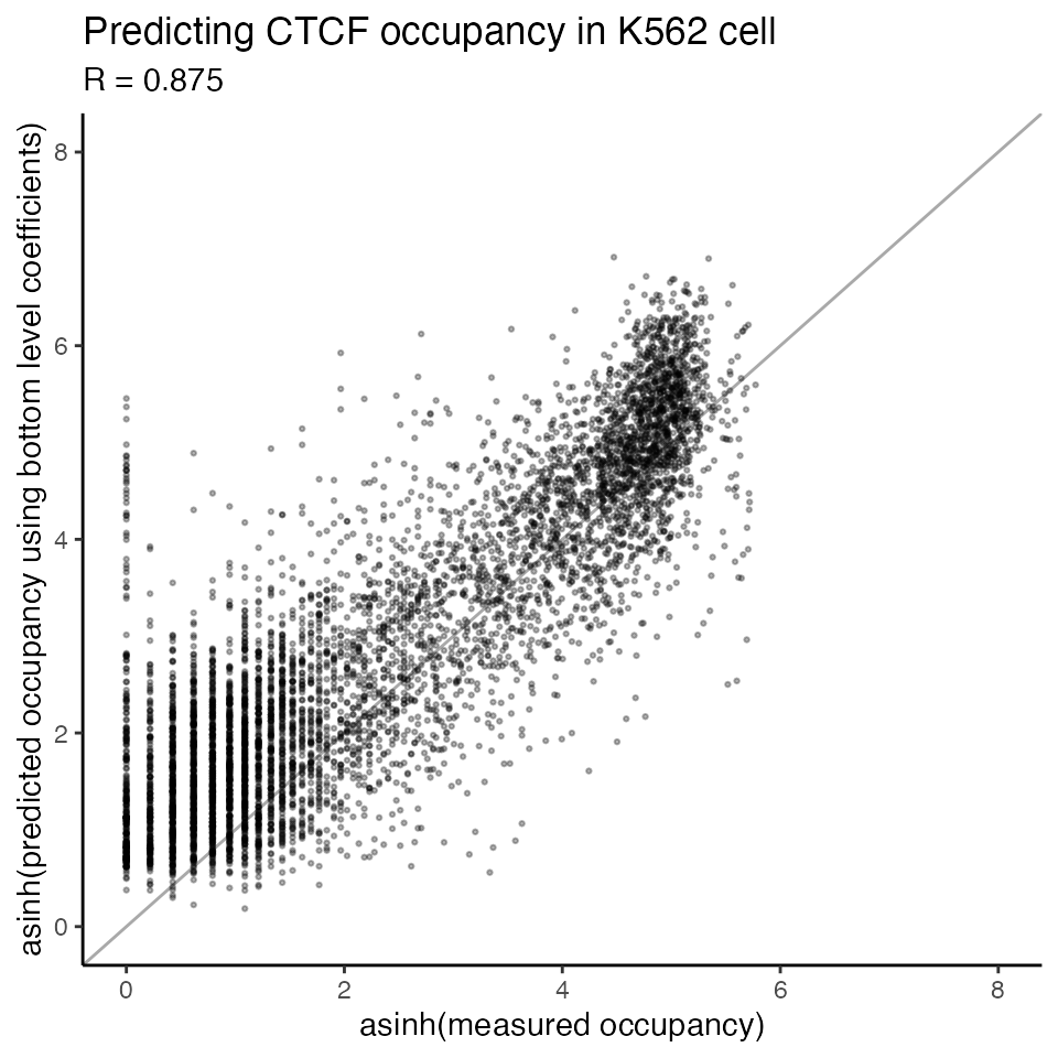
We can also try the “middle” level regression coefficients for CTCF, which are cell-type generic, thus could be used to predict CTCF in other cell types.
TOP_middle_result <- predict_TOP(data,
                                 TOP_coef = TOP_coef,
                                 tf_name = 'CTCF',
                                 level = 'middle',
                                 logistic_model = FALSE,
                                 transform = 'asinh')
#> Use the middle level model for CTCF.
#> Select features: pwm.score bin1 bin2 bin3 bin4 bin5
#> Predicting TF occupancy using TOP occupancy model...
TOP_middle_predictions <- TOP_middle_result$predictions
We can see the performance of the “middle” level model is very close to the “bottom” level model.
scatterplot_predictions(x = asinh(data_chip$chip),
                        y = asinh(TOP_middle_predictions$predicted),
                        title = 'Predicting CTCF occupancy in K562 cell',
                        xlab = 'asinh(measured occupancy)',
                        ylab = 'asinh(predicted occupancy using middle level coefficients)',
                        xlim = c(0,8),
                        ylim = c(0,8))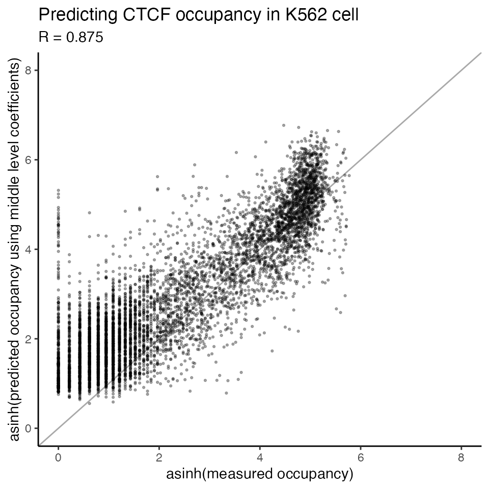
Predict TF binding probability using trained TOP logistic model
We can also predict TF binding probability for these candidate sites
using pre-trained TOP logistic model, by setting
logistic_model = TRUE.
TOP_result <- predict_TOP(data,
                          tf_name = 'CTCF',
                          cell_type = 'K562',
                          use_model = 'ATAC',
                          level = 'best',
                          logistic_model = TRUE)
#> Use pretrained TOP ATAC model coefficients ...
#> Use the bottom level model for CTCF in K562 cell type.
#> Select features: pwm.score bin1 bin2 bin3 bin4 bin5
#> Predicting TF binding probability using TOP logistic model...
logistic_predicted <- TOP_result$predictions
head(logistic_predicted, 5)
#>    chr  start    end  name pwm.score strand  p.value      bin1      bin2
#> 1 chr1  11122  11341 site1   22.4839      - 9.17e-09 0.2232134 0.0000000
#> 2 chr1  11180  11399 site2   20.7581      - 5.22e-08 0.0000000 0.2232134
#> 3 chr1  24681  24900 site3   16.5645      - 1.31e-06 0.0000000 0.0000000
#> 4 chr1  91319  91538 site4   15.1774      + 3.11e-06 0.2232134 0.2232134
#> 5 chr1 104884 105103 site5   15.6613      - 2.32e-06 0.0000000 0.0000000
#>        bin3      bin4      bin5   predicted
#> 1 0.0000000 0.0000000 0.0000000 0.061786177
#> 2 0.0000000 0.0000000 0.0000000 0.067183459
#> 3 0.0000000 0.0000000 0.0000000 0.014545759
#> 4 0.0000000 0.4361803 0.2232134 0.018758331
#> 5 0.2232134 0.0000000 0.0000000 0.009980625