TOP jointly fits a Bayesian hierarchical model using available training data from many TFs in many cell types.
Training TOP entails two basic steps, as illustrated in the figure below:
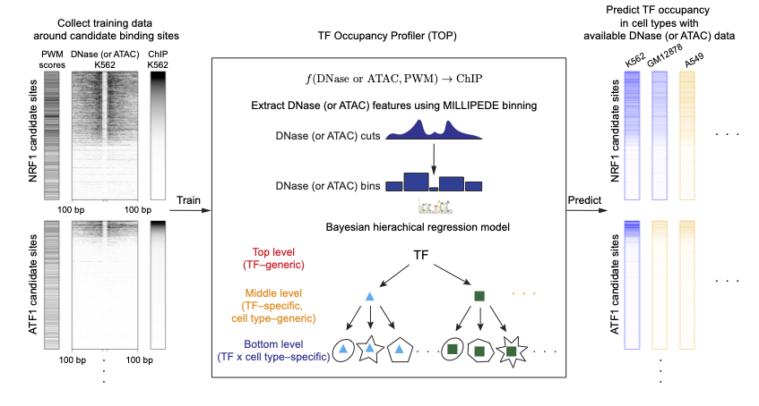
First, following the site-centric strategy, we use motif matches to enumerate candidate binding sites, and extract DNase- and/or ATAC-seq and ChIP data centered on each site for training.
Second, we fit our Bayesian hierarchical regression model on spatially-binned DNase- and/or ATAC-seq data.
Once TOP is trained, we can use it to predict occupancy for cell types or conditions for which we have DNase- or ATAC-seq data, generating TF occupancy estimates for ChIP-seq experiments that have not been done.
Load packages
We need to have R packages R2jags and doParallel installed in order to train TOP models, as we use JAGS to run Gibbs sampling for the Bayesian hierarchical model.
Prepare training data
As we learn the parameters from many TFs in many cell types together, it takes some efforts to prepare the training data.
Step 1: Prepare training data for each TF in each cell type
Firstly, we need to prepare training data for each training TF x cell
type combination, and save the training data files (as .rds
files in the data_file column in the table below).
This page shows the procedure to prepare the training data. Basically, for each TF in each cell type, we prepare training data for candidate binding sites: including: PWM scores of the motif matches, DNase (or ATAC) counts in 5 bins, and measured TF occupancy (from ChIP-seq data).
Step 2: Assemble training data for all TF x cell type combinations
We create a table (data frame) listing all training TF x cell type combinations. The table should have three columns: TF names, cell types, and paths to the training data files, like:
| tf_name | cell_type | data_file |
|---|---|---|
| CTCF | K562 | CTCF.K562.data.rds |
| CTCF | A549 | CTCF.A549.data.rds |
| CTCF | GM12878 | CTCF.GM12878.data.rds |
| NRF1 | K562 | NRF1.K562.data.rds |
| MYC | K562 | MYC.K562.data.rds |
| … | … | … |
In the example below, we split the training data randomly into 10 equal partitions, so that we could run Gibbs sampling on these partitions separately in parallel to reduce the running time.
We choose the training chromosomes by specifying the chromosomes in
training_chrs, for example using odd chromosomes as below.
The chromosome names (“chr…”) should match with those in the training
data.
assembled_training_data <- assemble_training_data(tf_cell_table,
                                                  training_chrs = paste0('chr', seq(1,21,2)),
                                                  n_partitions = 10)
Fit TOP quantitative occupancy models using assembled training data
Here, we fit TOP quantitative occupancy models with ChIP-seq read counts. To fit TOP logistic models with ChIP-seq binary labels, please see this tutorial.
We use the consensus Monte Carlo algorithm to run Gibbs sampling on each of the 10 training data partitions separately in parallel.
We first perform the “asinh” transform to the training ChIP-seq counts, then fit the TOP model to training data in each of the 10 partitions.
Set the following parameters for Gibbs sampling:
- n_iter: number of total iterations per chain (including burn-in iterations).
- n_burnin: number of burn-in iterations, i.e. number of iterations to discard at the beginning.
- n_chains: number of Markov chains.
- n_thin: thinning rate, must be a positive integer.
The following example fits a TOP model on all 10 partitions in
parallel using 10 CPU cores. It runs 5000 iterations of Gibbs sampling
in total, including 1000 burn-ins, with 3 Markov chains, at a thinning
rate of 2, and save the posterior samples to the TOP_fit
directory. It returns a list of posterior samples of the coefficients
for each of the 10 partitions.
It could take a long time if we have many TFs and many cell types in the training data.
all_TOP_samples <- fit_TOP_M5_model(assembled_training_data,
                                    logistic_model = FALSE,
                                    transform = 'asinh',
                                    n_iter = 5000,
                                    n_burnin = 1000,
                                    n_chains = 3,
                                    n_thin = 2,
                                    out_dir = 'TOP_fit')
If you have limited computing resource, you may fit model for each of
the 10 the partitions on separate machines, by specifying which
partition to run. For example, setting argument
partitions=3 will fit TOP model to the training data in the
3rd partition.
Combine TOP posterior samples from all partitions and extract the posterior mean of the regression coefficients
After we finished Gibbs sampling for all 10 partitions, we select and combine the posterior samples from all the partitions.
TOP_samples <- combine_TOP_samples(all_TOP_samples)
dim(TOP_samples)
We can extract posterior mean of the coefficients for all three levels.
TOP_mean_coef <- extract_TOP_mean_coef(TOP_samples,
                         assembled_training_data = assembled_training_data)
Save the posterior samples and posterior mean coefficients for predictions.
saveRDS(TOP_samples, 'TOP_fit/TOP_M5_combined_posterior_samples.rds')
saveRDS(TOP_mean_coef, 'TOP_fit/TOP_M5_posterior_mean_coef.rds')
We have included pre-trained model parameters using ENCODE data within this package, and also on our companion resources website. We will also train new models when new data become available, and update the model parameters on our companion site.
To make predictions for TF occupancy using new DNase- or ATAC-seq data using pretrained model coefficients, please see this tutorial.